FIU RCMI GIS Intermediate Workshop – Exercise 2

Exercise #2 -Analyzing point patterns in ArcGIS Pro

Objective: Learn how to geocode a table of addresses, analyze spatial patterns using spatial statistics, and interpret results.

This exercise gets you started with spatial statistics through a simple approach of analyzing point patterns. Similarly to how Dr. Snow plotted the addresses of cholera victims, we will start with a simple list of addresses. The detailed steps below walk you through the process.

Step 1 – Download data

• Download the dataset from here. The addresses_new.csv file contains 99 synthetic addresses from Miami-Dade County. These addresses were randomly generated and do not correspond to real people

Step 2 – Load and Geocode addresses

• Open ArcGIS Pro and create a new project called exercise_2.
• In the Map menu, click Add Data+ and find the addresses_new.csv file. You can also drag and drop the file from your file manager.
• Open the Attribute Table and verify the contents of the layer. Notice that the layer is recognized as a Standalone Table, which contains no geometries at this point.
• In the Analysis Menu, click Tools to open the Geoprocessing Toolbox. This is the main location from where different tools can be started.
• Search for the Geocode Addresses tool in the Geocoding Toolbox.
• Set the Input Table to addresses_new.csv, and the Input Address Locator to Esri World Geocoder.
• The software should automatically recognize that the input addresses are stored in different fields.
• Set the name and location of the Output Feature Class (optional).
• Choose United States as the Country or Region
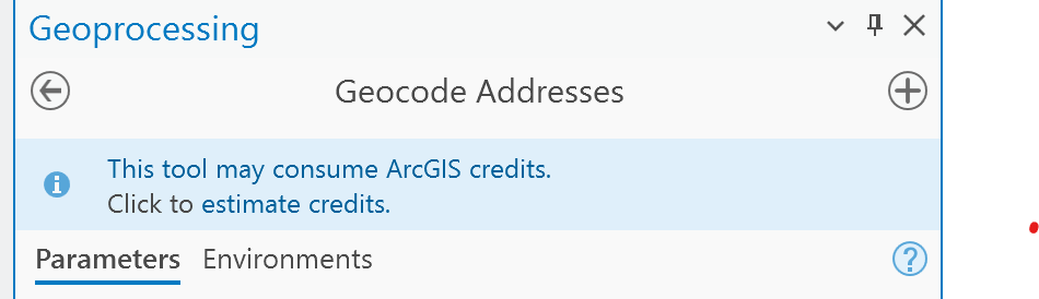
• Before you can Run the tool, you may need to click Estimate Credits highlighted in blue. This is because Geocoding is a premium service that requires a subscription. FIU’s institutional license allows each user to spend a certain amount of credits. This shouldn’t be an issue when working with reasonably sized datasets.

Step 3 – Perform Nearest Neighbor Analysis

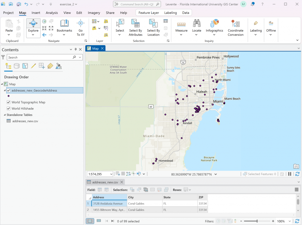
• Your screen should look similar to the one above, showing the location of addresses with point geometries.
• In the Analysis Menu (top) click Tools to open the Geoprocessing toolbox
• Find the Average Nearest Neighbor tool.
• Select the Input Feature Class and click the Generate Report checkbox.
• Locate the Report and open it (this will be a HTML file)

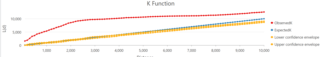
Step 4 – Ripley’s K function

• To calculate Ripley’s K function for our dataset, we need to Project the geographic coordinates into a projected coordinate system
• In the Analysis Menu (top) click Tools to open the Geoprocessing toolbox
• Open the Project tool
• Set the Input Feature Class to the geocoded addresses point layer
• Click the Globe icon next to the the Output Coordinate System field to open the selector window.
• Find Projected Coordinate System -> UTM -> North America -> NAD 1983 -> UTM Zone 17N (This is the Zone that covers Florida)
• After running the tool, you created a new layer from the geocoded addresses. Although both point sets appear at the same place on the map, the original layer stores geographic coordinates, whereas the new layer stores UTM coordinates
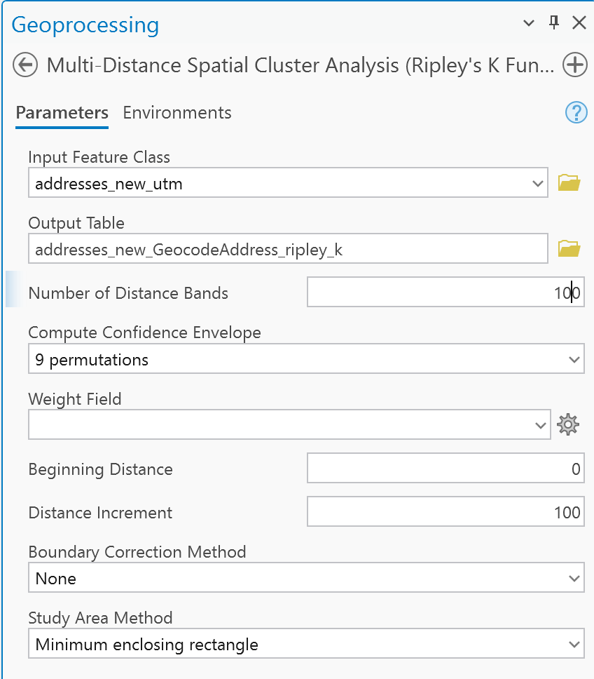
• In the Geoprocessing window, find the Multi-Distance Spatial Cluster Analysis (Ripley’s K Function) tool

Copy the parameters from below, then click Run.

• Check the table and Chart and see if you can interpret the results